TLDR

Wearable Fitness Trackers collect valuable data about the user that has the potential to be harnessed to predict user behavior and characteristics to facilitate self-understanding and behavioral change. This research project focused on conducting an N-of-1 study to predict an individual user’s duration of restorative night sleep, engagement in physical activity, and weight trend using wearable fitness tracker data of 401 days. Different variations of each model was run to explore the relationship between model output accuracy and model type, size of data, data split, data missingness, and data imputation. The possibility of outputting explainable predictions was also explored. The results showed that a Gradient Boosting model with non-imputed input data best predicted the sleep and physical activity target variables and a Gradient Boosting model with imputed input data best predicted the weight trend. This project acts as a preliminary investigative study into a field with many social, economic, and environmental implications which has the potential to improve the lives of individuals

1. Introduction

The Wearable Fitness Trackers (WFTs) market reached an all-time high of over 260 million users globally in 2023 and is projected to grow by 33% by 2028 [1]. Considering the fact that WFTs are designed to be worn all day for 24 hours, these devices collect valuable physiological and behavioral data about the user at an individual level. The primary goal of WFTs is to output fitness metrics such as caloric expenditure, steps taken, and average resting heart rate [2]. This research project investigates leveraging WFT data to accurately predict an individual’s behavior and characteristics in an explainable manner to facilitate self-understanding and behavioral change.

2. Problem Space Identification

To investigate the feasibility of the project and decide on tangible project goals and objectives, a thorough literature review was conducted to investigate prior research studies in similar domains. It was revealed that this research project falls under three prominent research domains, those being 1) N-of-1 research studies in healthcare, 2) user behavior or lifestyle prediction, and 3) WFT devices. Fourteen relevant articles were found across the three domains as seen in Figure 1.

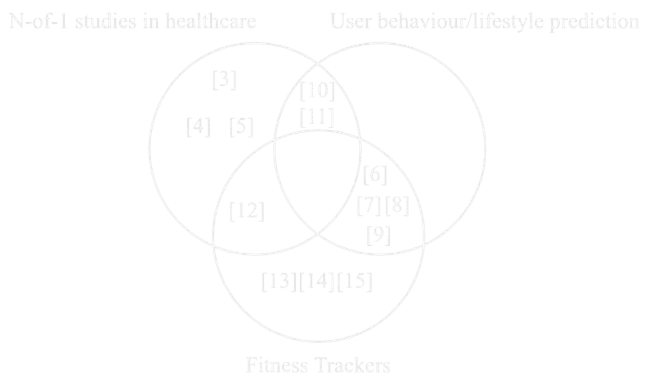
Figure 1. Research domains of literature review studies found

2.1 N-of-1 Healthcare Studies

A common finding from all N-of-1 healthcare studies reviewed is that such studies are important, efficacious, and useful in clinical healthcare, especially in delivering personalized healthcare [3][4][5]. Spieghelhalter in particular highlights that N-of-1 studies are more pragmatic and that conclusions drawn from such studies cannot be generalized to a population unlike typical N>1 studies [5] The literature reviewed in this domain provided a great overview of common statistical approaches used in N-of-1 studies such as time series analysis and provided a framework of to interpret findings and results of N-of-1 studies in a health-care context.

2.2 User Behavior and/or Lifestyle Prediction

A common approach in all the studies reviewed in the research domain of user action prediction is using aggregated personal data such as fitness data from WFTs or self-completed journals to predict a factor such as action compliance, behavioral patterns, and disease diagnosis for a population [6][7][8][9][10]. In the studies, a population is defined as a cluster of individuals grouped together based on a common, shared behavior such as daily activity levels. One of the key issues highlighted in this approach is the loss of crucial individual-level information due to data aggregation which might lead to inaccurate or incomplete conclusions [8]. Out of the reviewed literature, two studies by D. Lewis et al. [10] and B. Smith and P. Cunningham [11] shared similar objectives to this research project. D. Lewis et al. [10] built explainable AI (XAI) models using Shapley values to predict user engagement in mindfulness breathing habits based on self-completed journal entries. While the paper provided valuable insight and frameworks into building predictive XAI models, the paper lacked investigating data imputation strategies and its effects on model output which is a very important factor when working with real-life data. Similarly, B. Smith and P. Cunningham provided valuable insight into implementing AI models in an N-of-1 context by predicting runners’ best achievable race time using previous race times on a case-by-case basis, however, the study considered a very small number of input features, compared to WFT data, to get the final output [11].

2.3 Wearable Fitness Trackers

In this research domain, two studies investigated finding relationships between WFT data and user behavior such as periods of inactivity and user app usage [12][13]. While the articles highlighted important statistical considerations in such studies, the analysis conducted was not predictive. Moreover, one article concluded that WFTs have a satisfactory level of accuracy based on validation experiments conducted, keeping in mind that the studies utilized older models of WFTs that are no longer available for purchase [14]. Lastly, a study investigated WFT from a social point of view and highlighted the user privacy concerns associated with such devices [15].

3. Project Objectives and Timeline

Taking into consideration the project’s goal and the findings from the literature review, the project’s primary objective is to investigate whether any modern AI algorithm can accurately and consistently predict an individual user’s behavior and characteristics, in an explainable manner, with just the individual’s data available. The user behavior being predicted is the minutes of restorative night sleep a user will get the following day and whether or not the user will engage in physical activity the following day. The user characteristic being predicted is the direction of the user’s weight trend the following day (upwards or downwards). To clarify, the goal of the project is not to find one robust method that works across different individuals but rather to find a method that works for one individual consistently across time. Furthermore, the model’s predictions should be explainable to inform the user about which factors most contributed to the model’s prediction to facilitate user habit modification. Thus, the hypothesis tested in this project is that it is possible to use an AI algorithm to make useful predictions about an individual’s behavior and characteristics using an individual’s fitness tracker data only. More specifically the objectives of the project are as follows:

• Investigate the performance of different AI models for the prediction of each variable

• Investigate appropriate methods of splitting the available data into training, validation, and testing datasets

• Investigate the effects of data missingness and imputation on AI models’ performance

• Investigate the potential of leveraging XAI techniques to explain model outputs

With the final goal of finding the best AI model with an appropriate data split that most accurately predicts each of the three desired target variables, in an explainable way. The project’s timeline spanned thirteen weeks starting on January 27th, 2024. The first two weeks were dedicated to exploring the project’s overarching goals, assessing its feasibility, and adjusting the project’s scope based on feedback from the project advisor and course instructor. The following two weeks were used to conduct literature research and set concrete project objectives. The literature review stage was followed by four weeks of data collection, exploration, and cleaning which took longer than the anticipated one week due to unforeseen data export and structure issues which caused the project’s timeline to extend from twelve to thirteen weeks. This was followed by five weeks of multiple iterations of data modeling and result analysis. The remainder of the project was spent on finalizing the results and writing the project report.

4. Methodology

The methodology followed to meet the project objectives can be separated into five different phases: data collection and exploration, data cleaning and imputation, data splitting, modeling, and explainability.

4.1 Data Collection and Exploration

The personal data of the author of this paper, collected from the Whoop WFT and Withings smart scale was used for this project. The data collected included physiological, sleep, and workout data collected from the Whoop WFT, self-completed journal entries on the Whoop app, and weight data collected from the Withings smart scale from January 14, 2023, to February 28, 2024 (410 days). The details of the data included can be seen in Table A1 in Appendix A. Upon closer observation of the exported data, it was noticed that the in-app strength trainer that logs gym workouts, daily stress levels, and details of the journal entries were not available. For example, caffeine consumption was logged as a boolean value, without the amount of caffeine consumed. The Whoop customer support confirmed that there is currently no way of automatically retrieving this missing data. Therefore, the strength trainer data was manually entered as part of the workout data. The data exploration phase revealed high missingness (approximately 48%) in the journal data, except for the period between January 2023 and May 2023, as seen in Figure 2, and high missingness (around 67%) in weight data due to the user missing daily weigh-ins, respectively. The high missingness in journal data can be attributed to user negligence in filling out the journal and the frequent addition and removal of journal questions throughout the 14-month period. On the other hand, the other data columns had missingness of less than 1% (4 days) due to timezone discrepancies when traveling.

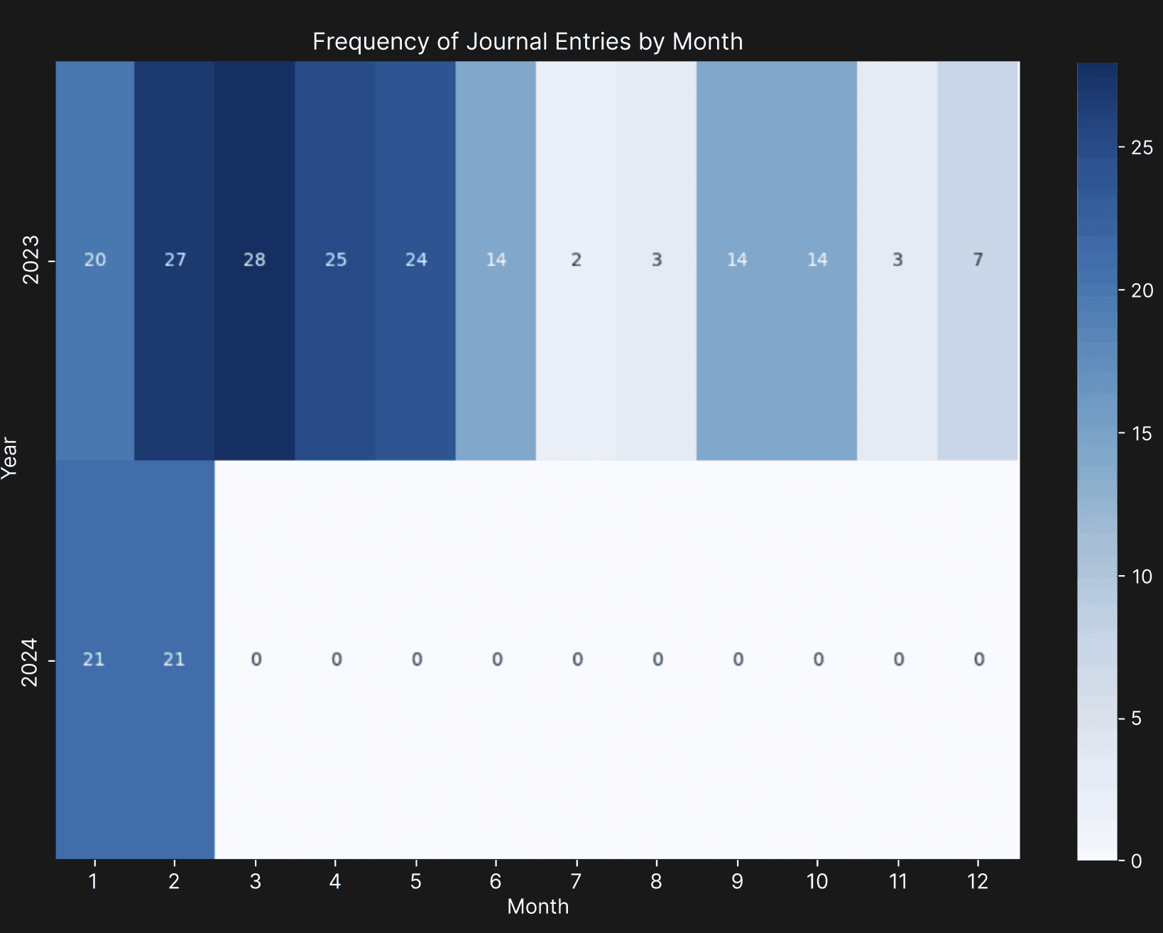
Figure 2. The density of journal entries from January 2023 to February 2024

4.2 Data Pre-processing

4.2.1 Data Cleaning

The major steps taken to clean the data to prepare it for model ingestion can be seen in Table 1.

Table 1. Major data cleaning steps done to pre-process the data

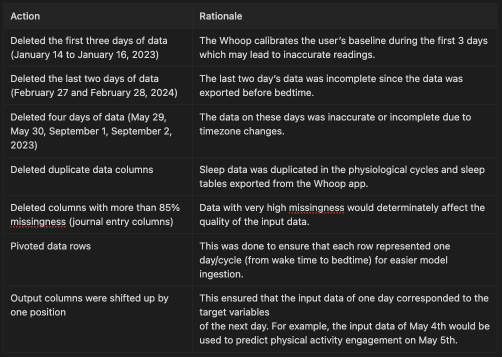
Action Rationale Deleted the first three days of data (January 14 to January 16, 2023) The Whoop calibrates the user’s baseline during the first 3 days which may lead to inaccurate readings. Deleted the last two days of data (February 27 and February 28, 2024) The last two day’s data was incomplete since the data was exported before bedtime. Deleted four days of data (May 29, May 30, September 1, September 2, 2023) The data on these days was inaccurate or incomplete due to timezone changes. Deleted duplicate data columns Sleep data was duplicated in the physiological cycles and sleep tables exported from the Whoop app. Deleted columns with more than 85% missingness (journal entry columns) Data with very high missingness would determinately affect the quality of the input data. Pivoted data rows This was done to ensure that each row represented one day/cycle (from wake time to bedtime) for easier model ingestion. Output columns were shifted up by one position This ensured that the input data of one day corresponded to the target variables of the next day. For example, the input data of May 4th would be used to predict physical activity engagement on May 5th.

4.2.2 Data Imputation

The missing journal entries were imputed using random hot-deck imputation, where missing values are replaced with randomly selected non-missing values from a donor pool (the rest of the data) [16]. This method was chosen since it is less sensitive to model misspecification and preserves data distribution [17]. The missing weight values were imputed using linear interpolation.

4.2.3 Extraction of Output Variables

To get the minutes of restorative sleep target variable, the minutes of deep and Rapid Eye Movement (REM) sleep, as detected by the WFT, were added together. The engagement in physical activity target variable was determined by whether or not the user completed a workout on a given day, which is automatically detected by the WFT or can be manually logged in on the app. The activity variable was given a value of 1 if the user engaged in physical activity, and 0 if not. The weight trend was computed by comparing the weight on a given day with the rolling weight average with a window size of 7. It is worth noting that using a window size of 7 resulted in all values being either -1 (downwards trend) or 1 (upwards trend) and no values of 0 (static weight) which meant that the task could be treated as a binary classification problem.

4.3 Data Splitting

4.3.1 Baseline and Full Datasets

Two datasets were constructed: a “baseline dataset” which included data from January 2023 to May 2023 (104 days) which only had approximately 10% missing journal entries and a “full dataset” (401 days) which included all of the data available which had around 48% missing journal entries. This was done to compare the performance of the models trained on data with low and missingness. Furthermore, two versions of each dataset were made, one with missing data and another with imputed data, which was done to compare the effect of data imputation on the performance of models that can handle null value inputs. The imputed baseline and imputed full datasets were imputed using case deletion and hot-deck imputation as mentioned previously, respectively. It is worth mentioning that as seen in Figures 3-5, the data distribution and balance remained relatively consistent between the baseline and full datasets except for the weight trend variable.

Figure 3. Data distribution of minutes of restorative sleep. (Left) in full dataset. (Right) in the baseline dataset.

Figure 4. Data distribution of physical activity engagement. (Left) in full dataset. (Right) in the baseline dataset.

Figure 5. Data distribution of weight trend. (Left) in full dataset. (Right) in the baseline dataset.

4.3.2 Training, Validation, and Testing Datasets

The data was split into training dataset, validation, and testing datasets in chronological order to ensure that only past data was used to predict future data. The sliding window technique, seen in Figure 6, was used for data splitting where the entire dataset gets sequentially partitioned into smaller training, validation, and testing datasets. In each iteration, the chosen window size determines the number of days used for each dataset and the step size determines how much the window moves forward in each iteration. The training window size was varied between 1 and 84 days, the validation window size was 25% of the training window size with a maximum of 5 days to ensure that recent data is used for training, and a testing window size of 1. The step size was strategically chosen to ensure that the sliding window traversed the entire dataset in evenly spaced increments in 5 iterations. For example, Figure 6 shows the five iterations of a training window of size 10 which corresponds to a validation window size of (10//4 =) 2, a testing window size of 1, and a step size of 26. In the first iteration, a model is trained on the first 10 days, validated on days 11 and 12, and tested on day 13. In the second iteration, the windows shift by 26 days and a new model is trained on days 27-36 (inclusive), validated on days 37 and 38, and tested on day 39. This pattern is then repeated 3 more times and the performance of the model at that training window size is averaged over the 5 iterations. This process is then repeated for all training window sizes. This data splitting method ensures that the data temporal relationships are maintained and that each model type is tested under a wide range of contexts. It is worth noting that the expanding window data split was with some of the models, but the sliding window data split was more appropriate since different days were used for testing, unlike the expanding window split which tested one day only.

Figure 6. Visual representation of the sliding window data splitting technique with a training window of size 10.

4.4 Modelling

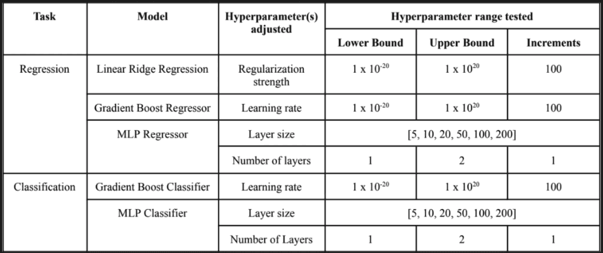
Linear regression, Gradient Boosting, and Multi-layer Perceptron (MLP) models were chosen due to their varying complexity (linear regression being the simplest and MLP the most complex) to investigate the trade-offs between model complexity, performance, and explainability. It is worth noting that the Gradient Boosting models can handle null values in the input data which was leveraged to assess the model’s performance with imputed datasets and datasets with null values. The performance for regressor models used for predicting minutes of restorative sleep were assessed using the Root Mean Squared Error (RMSE) value and the classification models used for the other target variables were assessed using the cross-entropy loss. Accuracy was not used since only one day is used for testing which yields an accuracy of either 0 or 1 in contrast to cross-entropy loss which considers the probability of a model outputting a correct prediction, thus providing a better comparative measurement to compare the performance of different models. Except for the hyperparameters seen in Table 2 all models were used with default parameter values in the Scikit-Learn model implementation [18]. Each model was trained on the training dataset at each training window size, the hyperparameter(s) tuned on the validation dataset, and its performance tested on the testing dataset. The MLP models however were trained, validated, and tested 5 times at each training window size due to the fluctuating output of the model that occurs due to randomized initialization of the parameter values. For MLP, the mean loss or error waere used for interpreting the model’s performance. Additionally, the linear regression model was only implemented for the regression task due to the tight project timeline and technical difficulties when implementing linear logistic regression for classification.

Table 2. The different models tested for each task and the hyperparameters tested on the validation data.

4.5 Explainability

To add explainability capabilities, Shapley values were leveraged due to their model-agnostic characteristic. Shapley values work by quantifying the marginal contribution of each feature to the output to aid in output interpretability [10]. For example, in the binary classification model for activity engagement, an input feature given a negative Shapley value indicates the feature’s association with a decreased probability that the user will engage in physical activity the following day by an amount equivalent to the magnitude of the Shapley value [10]. An advantage of this method is that the sum of values for all features represents the difference between the expected and predicted value, meaning that all input features are accounted for. The plan was to compute the Shapley values of the best-performing model for each of the target variables using the Shap Python package [19]. However, the Python package worked as expected for the simple linear regression model only, and returned Shapley values of 0 for all variables of the more complex models. Due to the tight project timeline, the Shapley values of the restorative sleep linear regression model only were computed.

5. Results

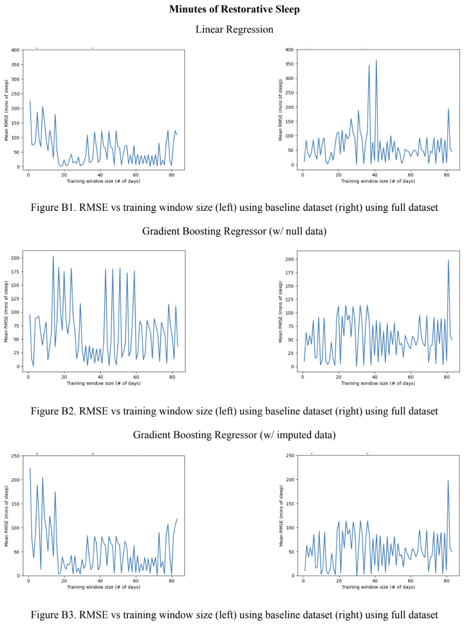
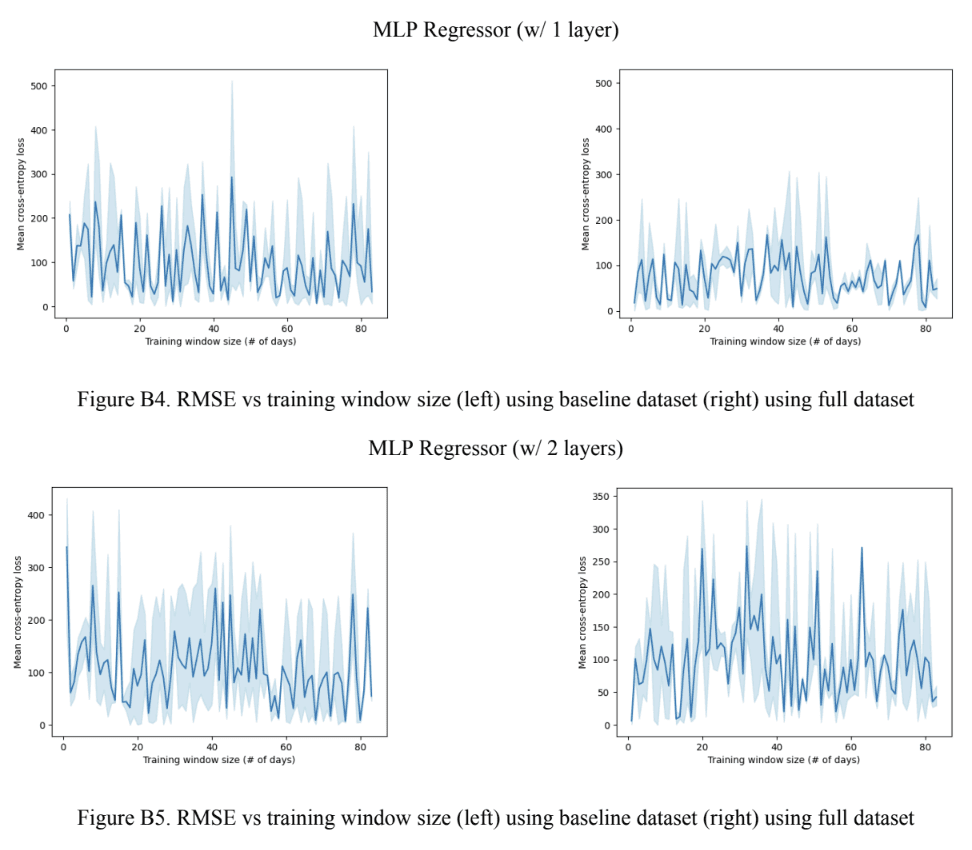
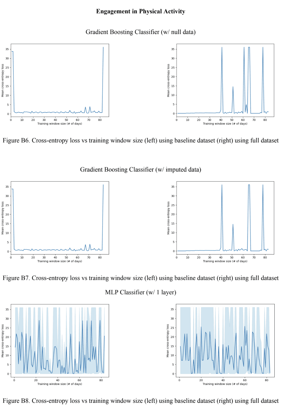
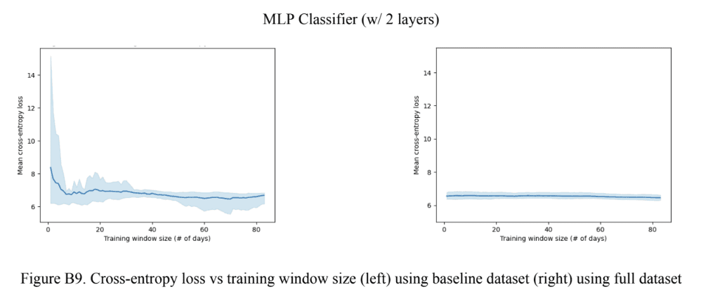
For each of the target variables, the mean error of the models across all training window sizes was compared to get a holistic view of each model’s performance with each of the target variables (Figures 7A, 9A, and 10A). To get a closer look at each model’s optimal performance to assess their potential in accurately predicting the target variable, the error at the best-performing (lowest error) training window size was compared as seen in Figures 7B, 9B, and 10B. To get an understanding of the data size requirements for each model, the training window size that produced the lowest error for each model was compared as seen in Figures 7C, 9C, and 10C. Lastly, the best-performing linear regression model for the restorative sleep target variable was re-run to get the Shapley values and assess the model’s explainability as seen in Figure 8. The plots for each model’s performance can be found in Appendix B.

5.1 Minutes of Restorative Sleep

Assessing the performance of the baseline regressor models across all training window sizes revealed a general positive correlation between the model’s complexity and error rate as seen in Figure 7A. This trend, however, is broken by the Gradient Boosting model using the imputed data which had the lowest RMSE out of all models. For the full models, it was found that the Gradient Boosting models outperformed both, the MLP models which performed the worst, and the linear ridge regression model. Taking a closer look at the Gradient Boosting models, it was revealed that the baseline models, the model using the dataset with the imputed values outperformed the one using the dataset with null values and vice versa for the full models. The 1-layer MLP model consistently outperformed the 2-layer MLP model. Looking at Figure 7B, no obvious trend between the the model complexity and optimal training window size for the baseline models was noticed. However, the optimal training window size stayed relatively consistent with all full models in the 20-30 range, except for the 1-layer MLP model which had an optimal training window size of 79. A similar trend was noticed with the full models where the RMSE was very close to 0 in all models, except for the 1-layer MLP, as seen in Figure 7C. For the baseline models, the Gradient Boosting model with null data had the lowest RMSE error and the 1-layer MLP had the highest.

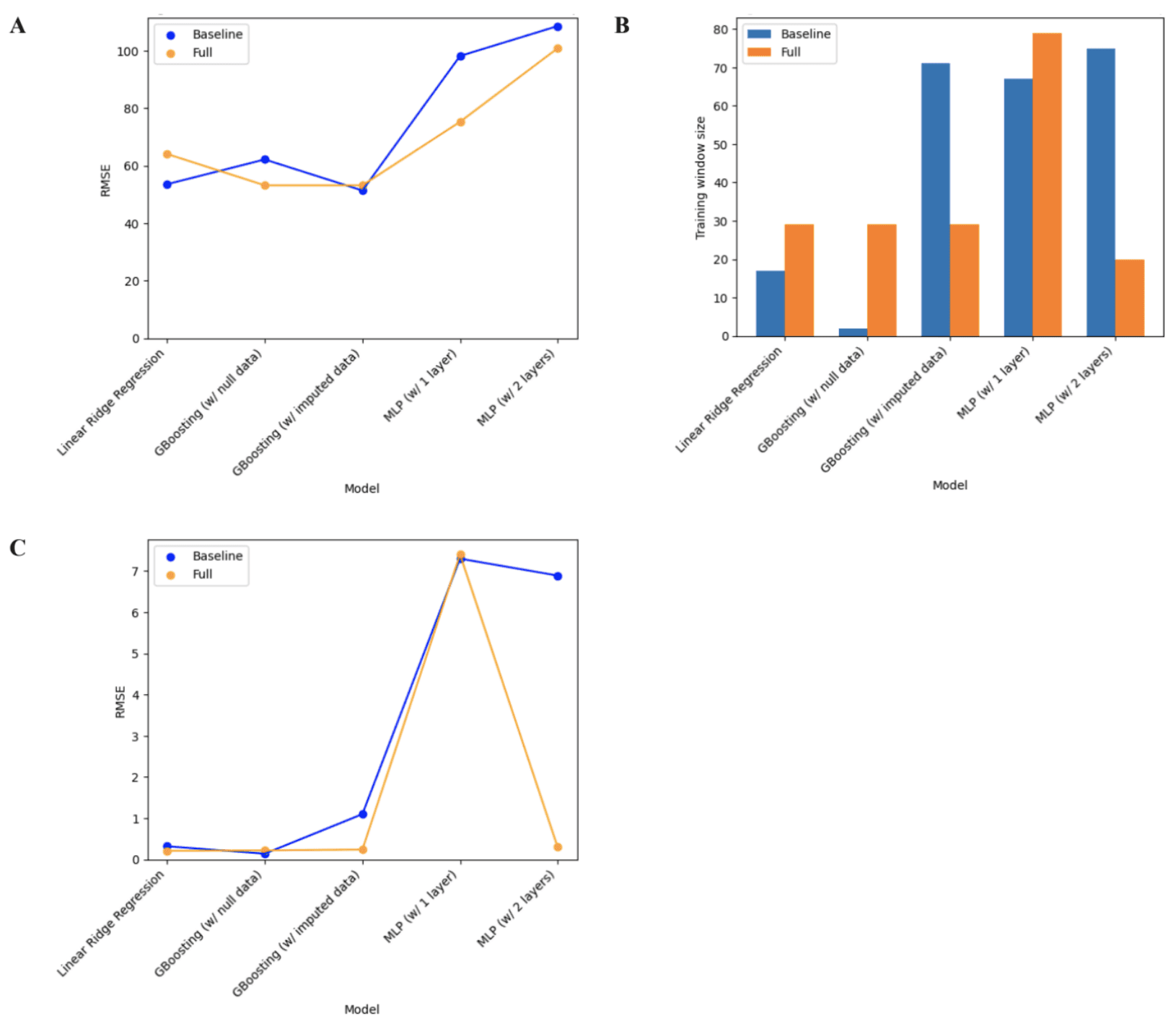
Figure 7. Regressor model performance (A) RMSE across all training window sizes. (B) Optimal training window size. (C) RMSE at the optimal training window size.

The best-performing model was considered to be the Gradient Boosting model using the null data which had the lowest RMSE value and small optimal training window sizes. Note that having a smaller optimal training window size is more favorable due to the smaller size of individual WFT datasets. The outputs of the Shapley values for the linear regression model, seen in Figure 8, indicate that the duration the user stays in bed, the strain on the user from physical activity, and the length of the user’s nap on a given day have the strongest positive associated with a longer duration of restorative night sleep. On the other hand, the maximum heart rate from physical activity, night sleep duration, and the sleep efficiency of naps have the strongest negative association with a longer duration of restorative night sleep.

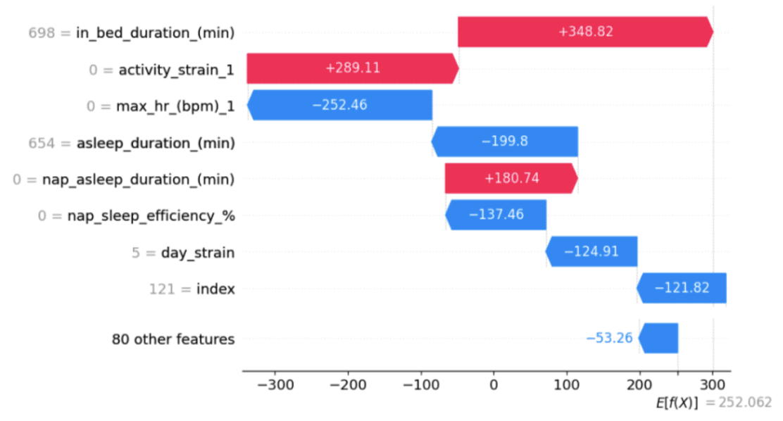
Figure 8. Waterfall plot of Shapley values for the linear regression model for predicting minutes of restorative sleep.

5.2 Engagement in Physical Activity

For the engagement in physical activity variable, the Gradient Boosting models outperformed the MLP models in all contexts as seen in Figures 9A and 9C. Upon closer observation of Figure 9A, it can be seen the Gradient Boosting model with null data outperformed the other boosting model for the baseline model, but not for the full model. A trend was observed in Figure 9C where the loss increased with model complexity (and also increased with using imputed data) for the baseline model, whereas the loss in the full models was relatively consistent at a value very close to 0, except for the 2-layer MLP which had a loss value 6.45. In terms of the optimal training window size, seen in Figure 9B, no particular trend was observed. However, a very small optimal training window size of 2 for the baseline Gradient Boosting model with null data was an interesting observation made. For the engagement in physical activity variables, the best-performing model was the Gradient Boosting model with the null data due to having the lowest mean cross-entropy loss and optimal training window size.

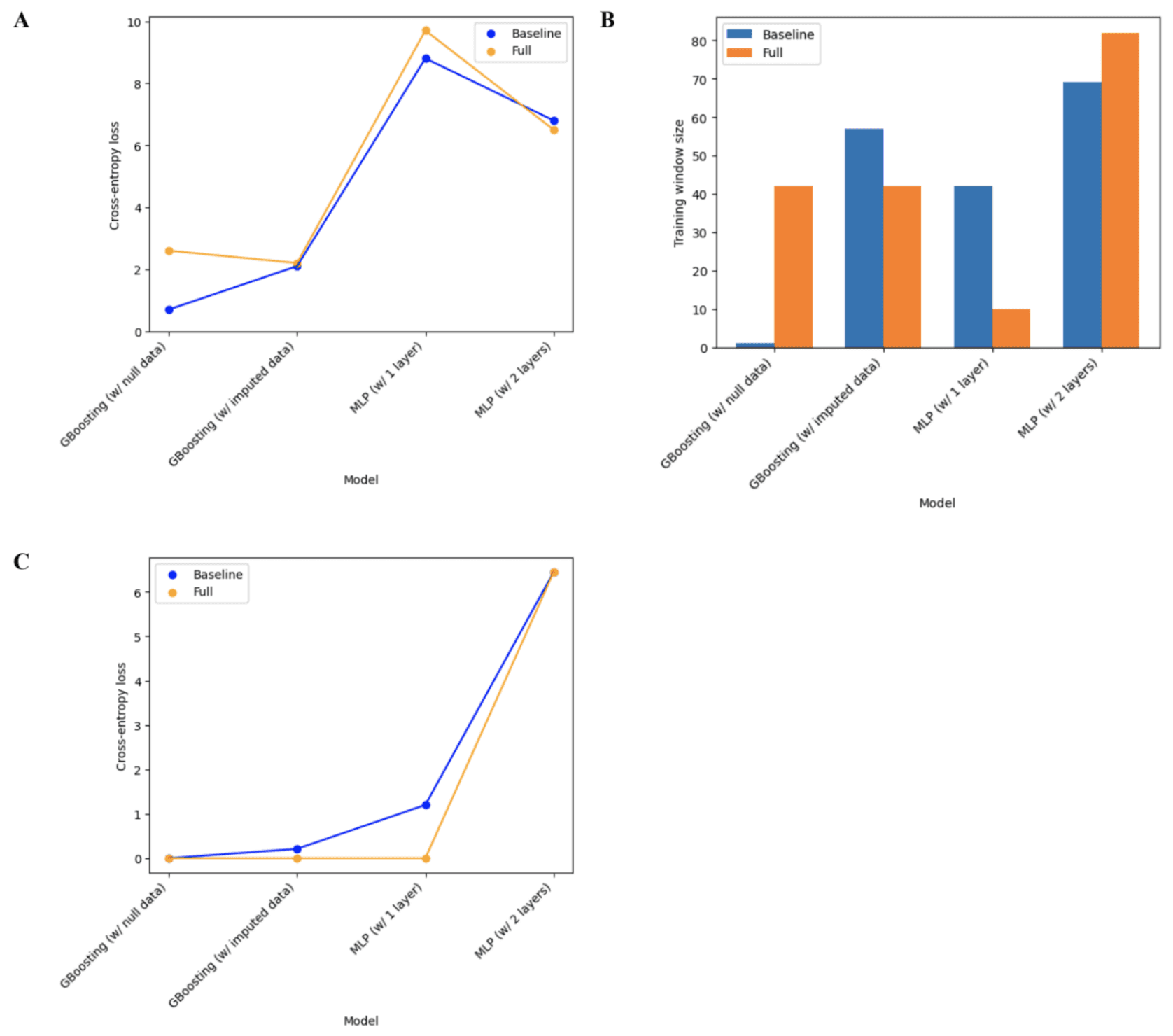
Figure 9. Classification model performance (A) Cross-entropy error across all training window sizes (B) Optimal training window size (C) Cross-entropy error at the optimal training window size.

5.3 Weight Trend

Through assessing Figure 10A, it was observed that all baseline models outperformed the full models for the weight trend variable. It is also worth noting that both the baseline and full 2-layer MLP models outperformed the 1-layer MLP models. For the Gradient Boosting models, the full model using imputed data slightly outperformed the full model using null data. This difference in performance was much more accentuated with the baseline model. Moving to Figure 10B, it was observed that the baseline Gradient Boosting models had a smaller optimal training window size compared to the baseline MLP models, but the opposite was true for the full models. Lastly, similar to Figure 9C, Figure 10A shows a cross-entropy loss very close to 0 for all full models except for the 2-layer MLP. The same can be said about the baseline model, however, both the 1-layer and 2-layer MLP had a significantly higher cross-entropy loss compared to the Gradient Boosting models. Based on these findings, it was concluded that the best-performing model with the Gradient Boosting model using the imputed data, by following the same criteria mentioned previously (mean cross-entropy loss and optimal training window size).

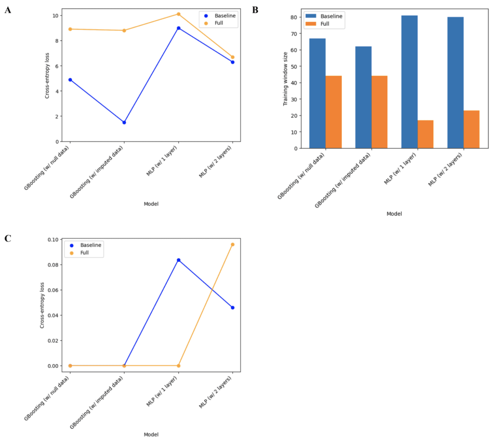
Figure 10. Classification model performance (A) Cross-entropy error across all training window sizes (B) Optimal training window size (C) Cross-entropy error at the optimal training window size.

6. Discussion

6.1 Model Complexity

All results for the variables demonstrated worse performance as the model used became more complex. This was the case when assessing the model’s mean loss across all training data window sizes, as well as the loss at the optimal training window size. The only exception to this behavior was the full Gradient Boosting model with the null data marginally outperforming the linear ridge regression model. This trend was expected since the more complex models require large datasets to avoid overfitting, which was not the case in the project. The complex models likely suffered from the curse of dimensionality due to the data’s high dimensionality (~100 input columns) and small size which made it harder for the model to accurately capture relationships in the data. To take it a step further, comparing the 1-layer MLP model to the 2-layer MLP model is not a fair comparison since the layer sizes are different for each model (determined by hyperparameter tuning on the validation dataset), thus determining which model is more complex would not be possible. Varying the number of layers was done to experiment with different MLP model architectures. Interestingly, this finding contradicts the study conducted by Lewis et al., where they found that more complex models were associated with more accurate prediction [10]. However, a direct comparison with Lewis et al. is not very appropriate due to the differing nature of data used (journal data vs WFT data, number of dimensions, etc.) and the different types of models used but is still a matter worth investigating further [10].

6.2 Dataset Size

When it comes to the dataset size required for the model to output the most accurate answer, it was hypothesized that the larger the size of the training data (i.e. larger training window) the lower the loss will be. However, this turned out to be a false statement since no obvious trend was seen that linked training window size with model output accuracy. A possible explanation for this phenomenon is the temporal relationship between the input and output data. In some cases, for trying to predict a future outcome, very old data would be irrelevant indicating that with time-series analysis, more data might not always be better.

6.3 Dataset Missingness

By comparing the performance of baseline models and full models on the mean loss across all training windows (Figures 7A, 9A, and 10A), a general trend can be seen where baseline models (that used data with low missingness) generally outperformed full models (that used data with high missingness) for classification tasks. This relationship was not present for the regression task where in the majority of cases (3 out of 5 models) the full model outperformed the baseline model (see Figure 7A). Seeing a trend where the model performs worse on data with more missingness is expected due to the absence of important information. However, further investigations are required to absence of the performance-data missingness relationship in the regression task. Unfortunately, no published literature were found that dealt with the effect of data missingness in a similar context during the literature review phase of the project.

6.4 Data Imputation

When comparing the two Gradient Boosting models using imputed data and data with null (non-imputed) values, a very similar performance (loss) can be seen in most cases (see Figures 7A, 7C, 9A, 9C, and 10C). The only exception to this trend is the mean loss across all training window sizes for the weight trend variable. A possible explanation for that discrepancy in performance between the classification of the weight trend (Figure 10A) and engagement in physical activity (Figure 9A) is the inherent differences in data balance between the two where the weight trend data is less balanced. Moreover, the data imputation does not seem to affect the optimal training window size when comparing Figures B6 and B7 in Appendix B. This does not come as a surprise due to the random nature of the imputation method used which tends to preserve data distribution. Another thing worth highlighting is that out of the three variables, the Gradient Boosting model with null data performed the best for two of the variables. This could be indicative of the slight negative impact the imputed journal data has on the models’ performance. Including the journal data might increase the negative impact of the curse of dimensionality. Taking all of this into consideration, it is fair to conclude that using random hot-deck imputation does not significantly affect the model’s performance.

6.5 Explainability

One thing that stands out when looking at the results of the Shapley values from the regression task in Figure 8 is the difference between correlation and causality. This means that it is up to the user to conduct further investigations to unlock causal relationships between inputs and the target variables. Leveraging Shapley values is a great technique for quantifying the effects of each variable on the output, however, in this case, it only worked for the linear regression model which is a very transparent model. This was unexpected since Shapley values are model-agnostic and have been implemented with more complex models in other research studies [10]. Further work must be conducted to understand why the Shapley values were 0 with the more complex (less transparent) models.

6.6 Summary of Findings

1. The best model for predicting minutes of restorative sleep was a Gradient Boosting Regressor with non-imputed, null data.

2. The best model for predicting engagement in physical activity was a Gradient Boosting Classifier with non-imputed, null data.

3. The best model for weight trend was a Gradient Boosting Classifier with random hot-deck imputed data.

4. The more complex models generally performed worse in predicting the target variables, likely due to the small, highly-dimensional input dataset used.

5. Providing more training data to the models does not necessarily improve its performance.

6. For classification tasks, input data with low missingness improved the models’ performance.

7. Random hot-deck imputation had a negligible effect on the performance of Gradient Boosting classifiers.

8. Explainable AI outputs provide correlational, rather than causal relationships between the input and output data.

Finally, it is worth noting that the primary limitation of this project is the lack of more robust testing to unlock more insightful data trends and explanations of observed phenomena which was due to a poor judgement of the project scope and available project timeline.

7. Project Implications

This project acts as an investigative research that intersects the three domains of N-of-1 healthcare studies, WFT data, and user behavior and characteristics prediction. As far as the author is aware, there are no other published research papers that tackle this research area. This project’s findings show promise in facilitating individual behavioral change by helping reduce the opacity around daily habits and behaviors, which would hopefully lead to individual lifestyle improvement. This leads to a healthier financial and social life due to a reduction in illness occurrence. Moreover, the individualized AI model approach reduces the models’ computational requirements which minimizes negative environmental impacts and increases user data privacy since the data is not reused to train other models. On the other hand, there are ethical concerns surrounding the potential emotional harm caused by predictive models, especially when dealing with sensitive topics such as health status. Inaccurate predictions such as a future upward weight trend, even though the user is following a strict diet or workout routine, for example, could potentially fuel the development of serious disorders such as eating disorders or body dysmorphia. This issue poses a great concern since similar phenomena have been reported by Whoop users when the data contradicted their expectations [20].

8. Conclusion and Future Work

This research project found that with the appropriate models, data split, and data imputation method it is possible to relatively accurately predict an individual user’s future length of restorative night sleep, engagement in physical activity, and weight trend. Further work is required to explore the possibility of outputting explainable model predictions to unlock causal relationships between daily habits and the target output variables. In future iterations of this research project, other areas that could be explored to reach more conclusive findings include additional feature selection to reduce input data dimensionality, exploring the prediction of the target variables for more than one day at a time, and conducting more testing to get explainable model output.

Acknowledgments

I would like to thank Dr. T. Stewart of the System Design Engineering Department at the University of Waterloo for the help, support, and guidance provided, as a project advisor, throughout the duration of the project. I would also like to acknowledge the efforts of Dr. M. Gorbet of Systems Design Engineering at the University of Waterloo for the valuable feedback and support provided during the project.

References

[1] Statista, “Global: fitness/activity tracking wristwear number of users 2019-2028 | Statista,” Statista, 2019. https://www.statista.com/forecasts/1314613/worldwide-fitness-or-activity-tracking-wrist-wear-users [Accessed Jan. 18, 2024]

[2] G. Shin et al., “Wearable activity trackers, accuracy, adoption, acceptance and health impact: A systematic literature review,” Journal of Biomedical Informatics, vol. 93, pp. 103153–103153, May 2019, doi: https://doi.org/10.1016/j.jbi.2019.103153.

[3] E. O. Lillie, B. Patay, J. Diamant, B. Issell, E. J. Topol, and N. J. Schork, “The n-of-1 clinical trial: the ultimate strategy for individualizing medicine?,” Personalized Medicine, vol. 8, no. 2, pp. 161–173, Mar. 2011, doi: https://doi.org/10.2217/pme.11.7.

[4] G. H. Guyatt et al., “Then-of-1 randomized controlled trial: Clinical usefulness,” Annals of Internal Medicine, vol. 112, no. 4, p. 293, Feb. 1990. doi:10.7326/0003-4819-112-4-293

[5] D. J. Spiegelhalter, “Statistical issues in studies of individual response,” Scandinavian Journal of Gastroenterology, vol. 23, no. sup147, pp. 40–45, Jan. 1988. doi: 10.3109/00365528809099158

[6] F. Gasparetti, L. Maria Aiello, and D. Quercia, “Personalized weight loss strategies by mining activity tracker data,” User Modeling and User-Adapted Interaction, vol. 30, no. 3, pp. 447–476, Jul. 2019, doi: https://doi.org/10.1007/s11257-019-09242-7.

[7] G. J. Martinez et al., “Predicting Participant Compliance With Fitness Tracker Wearing and Ecological Momentary Assessment Protocols in Information Workers: Observational Study,” Jmir mhealth and uhealth, vol. 9, no. 11, pp. e22218–e22218, Nov. 2021, doi: https://doi.org/10.2196/22218.

[8] T. Althoff, “Population-Scale Pervasive Health,” IEEE Pervasive Computing, vol. 16, no. 4, pp. 75–79, Oct. 2017, doi: https://doi.org/10.1109/mprv.2017.3971134.

[9] W. K. Lim et al., “Beyond fitness tracking: The use of consumer-grade wearable data from normal volunteers in cardiovascular and lipidomics research,” PLOS Biology, vol. 16, no. 2, pp. e2004285–e2004285, Feb. 2018, doi: https://doi.org/10.1371/journal.pbio.2004285

[10] R. Lewis, Y. Liu, M. Groh, and R. Picard, "Shaping Habit Formation Insights with Shapley Values: Towards an Explainable AI-system for Self-understanding and Health Behavior Change." CHI 2021 Workshop Paper. Realizing AI in Healthcare: Challenges Appearing in the Wild. May 2021.

[11] B. Smyth and P. Cunningham, “Marathon race planning: A case-based reasoning approach,” Proceedings of the Twenty-Seventh International Joint Conference on Artificial Intelligence, Jul. 2018. doi: 10.24963/ijcai.2018/754

[12] D. E. Rosenberg, E. Kadokura, M. E. Morris, A. Renz, and R. M. Vilardaga, “Application of N-of-1 Experiments to Test the Efficacy of Inactivity Alert Features in Fitness Trackers to Increase Breaks from Sitting in Older Adults,” Methods of Information in Medicine, vol. 56, no. 06, pp. 427–436, Jan. 2017, doi: https://doi.org/10.3414/me16-02-0043.

[13] T. Althoff, R. W. White, and E. Horvitz, “Influence of Pokémon Go on Physical Activity: Study and Implications,” Journal of Medical Internet Research, vol. 18, no. 12, pp. e315–e315, Dec. 2016, doi: https://doi.org/10.2196/jmir.6759.

[14] T. J. M. Kooiman, M. L. Dontje, S. R. Sprenger, W. P. Krijnen, C. P. van der Schans, and M. de Groot, “Reliability and validity of ten consumer activity trackers,” BMC Sports Science, Medicine and Rehabilitation, vol. 7, no. 1, Oct. 2015, doi: https://doi.org/10.1186/s13102-015-0018-5.

[15] M. B. Hoy, “Personal activity trackers and the Quantified Self,” Medical Reference Services Quarterly, vol. 35, no. 1, pp. 94–100, Jan. 2016. doi:10.1080/02763869.2016.1117300

[16] T. Emmanuel et al., “A survey on missing data in machine learning,” Journal of Big Data, vol. 8, no. 1, pp. 140-162, Oct. 2021. doi:10.1186/s40537-021-00516-9

[17] R. R. Andridge and R. J. Little, “A review of Hot Deck imputation for survey non‐response,” International Statistical Review, vol. 78, no. 1, pp. 40–64, Apr. 2010. doi:10.1111/j.1751-5823.2010.00103.x

[18] SciKit-Learn, “scikit-learn: machine learning in Python — scikit-learn 1.4.2 documentation,” Scikit-learn.org, 2024. https://scikit-learn.org/stable/ [Accessed Apr. 28, 2024].

[19] SHAP, “Welcome to the SHAP documentation — SHAP latest documentation,” Readthedocs.io, 2018. https://shap.readthedocs.io/en/latest/ [Accessed Apr. 28, 2024].

[20] ABR-reddit, “My experience after using whoop for more than 1 year,” Reddit.com, 2024. https://www.reddit.com/r/whoop/comments/1bh11u2/my_experience_after_using_whoop_for_more_than_1/ [Accessed Apr. 27, 2024].

Appendices

Appendix A

Table A1. Metadata of Whoop’s exported data.

Column Name (Data Type/Unit)

General

Cycle start time (Time), Cycle end time (Time), Cycle timezone (Time)

Journal Data

Consumption of processed foods (Y/N), Consumption of fruits or vegetables (Y/N), Eating close to bedtime Boolean (Y/N), Experiencing irritability (Y/N), Experiencing seasonal allergies (Y/N), Experiencing sadness (Y/N), Feeling recovered (Y/N), Consumption of caffeine (Y/N), Adequate hydration (Y/N), Fasting (Y/N), Tracking calories (Y/N), Working from home (Y/N), Commuting to work (Y/N)

Physiological Data

Recovery score (%), Resting heart rate (Beats per minute), Heart rate variability (Milliseconds), Skin temperature (Degrees celsius), Blood oxygen level (%), Day Strain (Float), Energy burned (Calories), Maximum heart rate (Beats per minute), Average heart rate (Beats per minute)

Night Sleep Data

Sleep onset (Time), Wake onset (Time), Sleep performance (%), Respiratory rate (Respirations per minute), Asleep duration (Minutes), In bed duration (Minutes), Light sleep duration (Minutes), Deep (SWS) sleep duration (Minutes), REM sleep duration (Minutes), Awake duration (Minutes), Sleep need (Minutes), Sleep debt (Minutes), Sleep efficiency (%),Sleep consistency (%)

Nap Sleep Data

Nap onset (Time), Nap wake onset (Time), Nap sleep performance (%), Nap respiratory rate (Respirations per minute), Nap asleep duration (Minutes), Nap in bed duration (Minutes), Nap light sleep duration (Minutes), Nap deep (SWS) sleep duration (Minutes), Nap REM sleep duration (Minutes), Nap awake duration (Minutes), Nap sleep need (Minutes), Nap sleep debt (Minutes), Nap sleep efficiency (%)

Physical Activity

Workout start time (Time), Workout end time (Time), Duration (Minutes), Activity name (String), Activity strain (Float), Energy burned (Calories), Maximum heart rate (Beats per minute), Average heart rate (Beats per minute), Heart rate zone 1 (%), Heart rate zone 2 (%), Heart rate zone 3 (%), Heart rate zone 4 (%), Heart rate zone 5 (%), GPS enabled (Y/N), Distance (meters), Altitude gain (meters), Altitude change (meters)

Appendix B

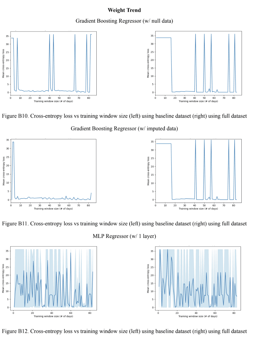
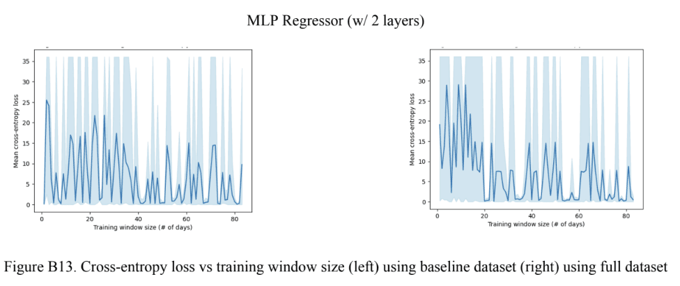
Note: the shaded region in the MLP plots represents the maximum and minimum values at each training window size. The line represents the mean.