RNA Neucleotide Reactivity Prediction
Statement of Individual Contribution
This project was a group effort of 4 members (including me). My primary responsibilities were pre-processing the data to prepare it for model consumption which included figuring out the type of processing required, writing the Python script, and testing it. I also wrote the Optuna code for hyperparameter space exploration which was used by each group to run the script and divide the computational load amongst group members. Furthermore, I contributed to literature research, report writing, and running the final model with the chosen hyperparameters.
TLDR
This paper presents an encoder transformer model for predicting RNA folding given different sequences and reactivities when presented with 2 different chemical reagents added. Understanding how RNA folding works is key to several new discoveries and techniques in the medical field that cannot be solved on a protein level. It would be extremely advantageous for a deep learning model to accurately predict these mechanisms to assist researchers and scientists in making a breakthrough.
Data provided on Kaggle regarding the reactivities, sequences, and experiment types were preprocessed, mapped accordingly, and split between three sets of data. Several different architectures were studied extensively with several different variable parameters from dropout, encoder heads, encoder layers, and model dimensions were extensively investigated with different learning rates. A sinusoidal positional embedding was used for the given model dimension in the RNATransformer. Optuna was used for tuning the parameters following a manual parameter investigation. MAE loss was utilized as the performance metric and an 8.5% reduction in test loss was observed in the final model application.
1. Introduction
An important feature of ribonucleic acid (RNA), an essential biological molecule, is its ability to fold into complex secondary and tertiary structures to execute critical biological functions [1, 2]. The current and future understanding of RNA is of extreme interest to scientists because understanding RNA is the key to large medical advances in finding cures for pancreatic cancer, Alzheimer's, and various other bacterial, neurological, cancerous, or viral diseases [1]. Each RNA molecule is single-stranded and made up of four bases along the singular helix: adenine (A), uracil (U), cytosine (C), and guanine (G) [1]. These RNA bases then form sets of base pairings to form 2D RNA structures and may interact further to form 3D tertiary structures [3]. The sequence of the bases in the RNA results in different foldings to chemical reagents where their reactivities can be predicted and the process of RNA folding better understood [1]. The folding process can be represented in terms of where these bases connect to make folds [1].
The goal of the project is to predict the chemical reactivity of each base in different sequences to develop a stronger understanding of RNA structure for possible future medical advances [1]. How the folding mechanism works in RNA when exposed to chemical reagents is immediately useful for medical breakthroughs in developing mRNA vaccines, CRISPR therapeutics and shows potential to open avenues to medical disease solutions that scientists cannot treat on a protein level [1]. The Kaggle competition provided a comprehensive training dataset for two reagents: 2-aminopyridine-3-carboxylic acid imidazolide (2A3) and Dimethyl sulfate (DMS), sequences of RNA strands and the resulting expected reactivities with some additional information on the RNA functionality [1].
2. Literature Review
2.1 RNA Chemical Probing
Chemical probing has been proven to be an effective technique for RNA structural analysis [2]. Dimethyl sulfate (DMS) has traditionally been used as a probing reagent which allowed high-throughput measurements of RNA base-pairing in living cells [4]. However, this approach worked well for adenine and cytosine bases but faced challenges with uracil and guanine bases until the development of four-base DMS-MaP which solved this problem and successfully conveyed more in-depth structural information [4][5]. Furthermore, 2-aminopyridine-3-carboxylic acid (2A3) chemical probing has been shown to outperform other state-of-the-art RNA structural analysis techniques and shows promise for both in vitro and in-vivo structural RNA analysis [6]. Overall, both techniques have been revolutionary in our understanding of RNA’s structure and behavior, however, still have room for improvement in terms of the structure’s resolution [7].
2.2 Deep Learning Techniques in RNA Prediction
Multiple Deep Learning models have been implemented in RNA structure identification and formation predictions due to their ability to extract and decipher underlying relationships from large amounts of data [6]. There have been multiple successful implementations of Deep Learning in the context of RNA including Wang et al.’s (2023) successfully implemented a transformer model to predict 1D and 2D RNA geometrics which outperformed traditional and other deep-learning methods, Franke et al. (2023) achieved state-of-the-art performance by leveraging transformer-like axial attention architecture to predict RNA secondary structures, He et al. (2023) used transformer encoders to accurately predict mRNA degradation at a nucleotide level, and Booy et al. (2022) used convolutional networks to predict RNA base pairings [8][9][10][11]. That being said, model overfitting is a common issue hindering the success of these implementations due to models’ high complexity and the limited amount of RNA structure data availability [7]
3. Methodology
3.1 Model Choice
Given the nature of the problem, Recurrent Neural Networks (RNNs) and more specifically Long Short-Term Memory models (LSTMs) would be an obvious choice due to their ability to capture long-range dependencies in sequences such as the RNA sequence and capture the complex relationships between the nucleotides [12]. However, it was decided to proceed with an encoder-only transformer due to several advantages it provided over LSTMs which include:
Transformers’ self-attention mechanism and positional encodings enable the model to capture long-range dependencies between nucleotides in the sequence effectively [13].
Due to the absence of recurrence in transformers, it will not suffer from vanishing gradients [14]
Due to the limited 30-hour GPU runtime availability on Kaggle, transformers were preferred due to their ability to process the RNA sequences in parallel rather than sequentially which makes them more computationally efficient [13].
Furthermore, pieces of literature show promise for the success of transformers and transformer-like structures in the context of RNA as previously discussed in the literature review section of this report. All things considered, it was decided to move forward with an encoder-only transformer model due to its attention mechanism and previous research conducted that showed promise for a successful model.
3.2 Data Pre-processing
To start off, the data in the ‘train_data_QUICK_START.csv’ file provided in the Kaggle competition was processed to prepare it for ingestion by the model. It is worth noting that this csv file was used rather than ‘train_data.csv’ since the former file was filtered based on the signal-to-noise ratio. This means that the file has better-quality data for the model to train on, however, the main drawback is that it has less data (335616 rows in the quick_start csv compared to 1643680 in the other file) but the available data in the quick start file is sufficient to build a well-performing model which will be discussed in more detail in the Results and Discussion section of this report. To prepare the data for use by the model, the following pre-processing steps were taken:
Mapped each base in the RNA sequence to a numerical integer value between 1 and 4
Mapped the experiment type to a numerical value, either a 1 or a 2
Duplicated the numerical experiment type so that its length matched the length of the associated RNA sequence length
Added a right padding of zeros to shorter RNA input sequences to ensure that all sequences are of the same length
Added a right padding of zeros to shorter experiment type sequences to ensure that all sequences are of the same length
Filled empty values (i.e. NaN values) in the reactivity output with a 0
Added a padding mask to mark the positions of the padded elements in the RNA input sequence and experiment type sequence
The result of these data pre-processing steps was a dictionary of data with RNA sequence inputs, experiment types, and reactivity targets. This dictionary was then used to set up a custom torch-style dataset to make it streamline the process of working with the data with the Pytorch models. Furthermore, the data was split into 64% training data (214793 rows) used to train the models, 16% validation data (53699 rows) used to tune the model’s hyperparameters, and 20% testing data (67124 rows) used to assess the performance of the final optimal model on unseen data. Before the initialization of the model, a batch size of 128 was utilized to gather data from the training, validation and test results.
3.3 Model Initialization
The encoder-only transformer covered in Tutorial 8.1 was used as a starting point. A sinusoidal positional embedding was also created corresponding to the length of the RNA strand sequence (206) and the dimension of the model (variable). An encoding layer using ‘GELU’ nonlinearity was created using the variables input, and a linear layer is created of model dimension to model dimension before the model adds the final neurons*final weights to retrieve the resulting reactivity. Dropout layers are added for the encoder and the linear layer to add robustness to the model over iterations as well as regularize the output. The mean squared error (MSE) was used as the loss function to minimize via backpropagation and MAE loss was used as a performance assessing metric for every epoch. The model trains on data in the training set, explores the hyperparameter space using the validation set, and retrieves final results using the test set.
3.4 Hyperparameter Exploration
In order to minimize the test error, we explored different architectures, optimization, and regularization methods based on the most relevant hyperparameters for our transformer architecture. Data augmentations such as random nucleotide replacement, deletion, or insertion were not applied due to the very complex nature of RNA structures and base interactions. Such data augmentations may introduce biologically implausible RNA sequences that may significantly affect the reactivity output values, thereby hindering the model’s learning process. Additionally, since data augmentations run on CPU rather than GPU, this would have slowed down the exploration process significantly [15].
In addition, the ADAM optimizer was used for all experiments with optimized parameters due to its general high effectiveness in industry [16]. The number of epochs used varied between experiments dependent on learning rate, runtime, general performance evaluation, and available GPU resources at the time. With that in mind, the following hyperparameters were selected for exploration.
Architecture: Number of heads, Model dimension, and Number of layers
Regularization: Dropout rate and Early-Stopping
Optimization: Learning rate
The initial run used the following hyperparameters:
Number of heads: 4
Model dimension: 128
Number of layers: 3
Dropout rate: 0.1
Learning rate: 1e-3
Early-stopping: Not applied
These values were the baseline for the hyperparameter optimization. At 5 epochs, our model achieved a test error of 0.14558 using the hyperparameter values above. This was the starting point for mean squared error loss, and the goal was to improve this error value both with manual exploration and automatic Optuna optimization.
First, manual exploration was performed to examine how each hyperparameter affected the model’s performance. Manual exploration was done by changing only one hyperparameter per run and checking how the model’s performance changes. Both larger and smaller values than the initial architecture were checked. For example, to test how the dropout rate affects the model’s performance, an experiment was run with dropout rates larger than 0.1 and with rates lower than 0.1. The optimal range for each hyperparameter was then determined based on the results of these experiments and used for Optuna optimization which will be discussed in further detail in the next section of this report. **After running an Optuna study with 10 trials and 5 epochs per trial, the best-performing hyperparameters were used to build a final model that was trained on the training data and its generalizability assessed on unseen test data. It was decided to carry out 10 trials of 5 epochs each due to the limited GPU resources available after an extensive manual hyperparameter space search, which was believed to be enough to assess the effects of the hyperparameters on the model’s performance.
3.5 Model Assessment to Baseline
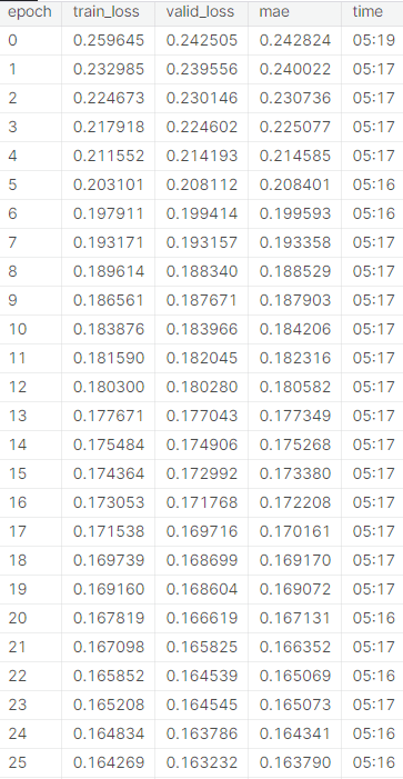
Another model was found online, built by Kaggle user “Iafoss” to be used as a baseline to quantify the progress made in the final model early into the competition [17]. The baseline model uses an encoder setup and sinusoidal position embedding with pre-sorted/premodified data similar to our usage of the ‘train_data_QUICK_START.csv’. The baseline model utilized mini batching to input data, which increased epoch speed while training for similar trends among data. The baseline model is extremely similar to the final model, but did not utilize Pytorch, and was less computationally complex. The baseline model originally outputted a final MAE test loss of 0.163128 after 32 epochs (and 0.163790 after 25 epochs which we will be using for comparison). When modified to train for MSE, the model performed worse than initially for MAE loss (prioritized MSE test loss too effectively). Therefore, the test loss that we will be comparing our model is 0.163790 (original method over 25 epochs). The relevant results can be seen in the appendix for training/test loss per epoch.
4. Results and Discussion
4.1 Manual Hyperparameter Exploration
Table 3 shows the experiments done for manual exploration. The base model is shown in light blue, models that resulted in a better performance are shown in green, and modes with worse performance in yellow. The results and discussion for the optimal ranges for the manual hyperparameters exploration were the following:
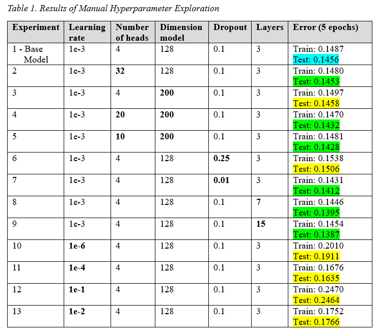
Model dimension: A model dimension range from 32 - 200 was explored. It was discovered that the larger the model dimension, the lower the training and test MSE loss was, as expected. Furthermore, it was discovered that the ratio of model dimension to number of heads is more relevant to the model’s performance than each individual value by itself. Therefore, an optimal ratio (model dimension / number of heads) was found to be between 10 and 30. Therefore, it was concluded the ideally the final model would have the largest possible (206) model dimension value that is divisible by the number of heads (using the optimal ratio).
Number of heads: An even number of heads in the range between 2 and 50 was explored. As mentioned previously, the model dimension to number of heads ratio was more important than the number of heads. Therefore, we found that the optimal range for the number of heads was between 6 and 20 heads. This range was calculated using the optimal ratio which was found to be 10-30 and the maximum number for the model dimension. The calculation for model dimension and number of heads looked as follows in pseudo code:
Number of Layers: For the number of layers, a range between 3 and 10 layers was considered. An upper bound of 10 layers was placed due to the very slow model training runtime when the number of layers exceeded 10 and the considerably low MSE test loss as seen in Table 1. Since a larger number of layers yielded a lower training and testing loss, it was decided to not include this hyperparameter in the Optuna study since its behavior was found to be predictable and consistent.
Dropout rate: A dropout range from 0.01 - 0.50 was explored. Contrary to the team’s expectations, higher dropout rates seemed to yield larger training and testing loss values (poorer performance) likely due to model underfitting. As a result, the optimal range for dropout rate was found to be between 0.01 to 0.1.
Learning rate: The initial learning rate of 1e-3 was used resulting in good results. Further experimentations with learning rates between 1e-1 and 1e-6 were conducted. Both ends of the exploration bounds yielded worse results (lower testing accuracy), indicating the optimal range for learning rate was close to the initial guess. The optimal range was from 0.55e-3 to 5.5e-3.
Early-Stopping: Early stopping is effective for preventing the model from overfitting. This hyperparameter was not investigated since the model did not overfit. This could be explained by the short 5 epoch runs conducted which is a short span to encounter overfitting. However, in longer runs, early stopping may be required and will therefore be implemented in future models.
Weight Decay: 1e-6 was used for some experiments with higher epochs as the effect of weight decay was minimal with lower epoch experiments and could slow the exploration process of the hyperparameters.
4.2 Optuna Study Results
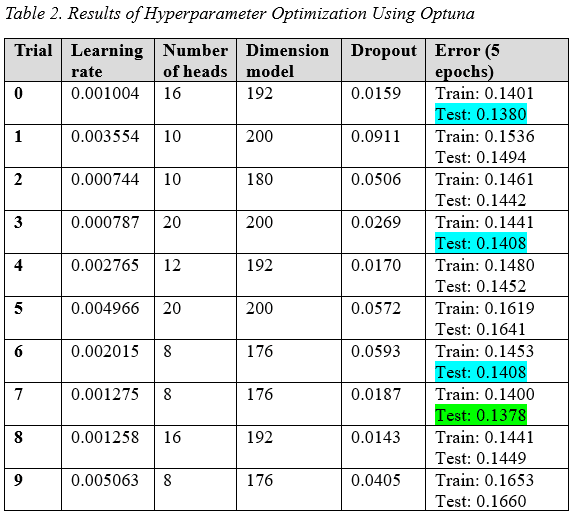
After the manual hyperparameter space exploration, Optuna was utilized to find appropriate hyperparameter values. The specific hyperparameter values and their associated ranges can be found in Table 2. The best result is shown in green, and other satisfactory results in blue.
It was observed that the best result (lowest testing loss) found with Optuna was better than all the results obtained through manual exploration. Furthermore, for the Optuna study, the number of layers was constant (3 layers) for all trials to save GPU runtime since it was known that increasing the number of layers would improve the model’s performance. For the final model, the number of layers will be increased from 3 to 10 to further improve the model’s performance.
4.3 Final Model Implementation
The final encoder-only transformer model was trained on batches of the training data and then tested on unseen test data using the best hyperparameters found via the Optuna study. This new and additional mini batching step was introduced to ensure that the model processes a new data batch each epoch and learning rate scheduling for the Adam optimizer was introduced at intervals where convergence began to slow down significantly. The minibatch size was set to be equivalent to the model dimension and learning rates decreased by a factor of 10 at the intervals to speed up the gradient descent once the model approached the local minimum. The results of the experiment are seen in Table 3. Mini batching was utilized similar to the baseline implementation to ensure that new batch data was processed during each epoch (rather than training on the same batch for the duration to accurately depict the full training/testing set of data).
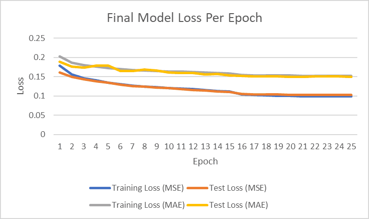
Figure 1: Final model performance for training and test loss (MSE and MAE)
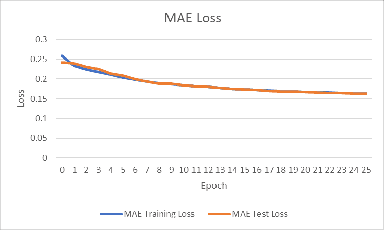
Figure 2: Baseline mode performance for training and test loss (MAE)
Table 3. Training and testing metrics of the final model
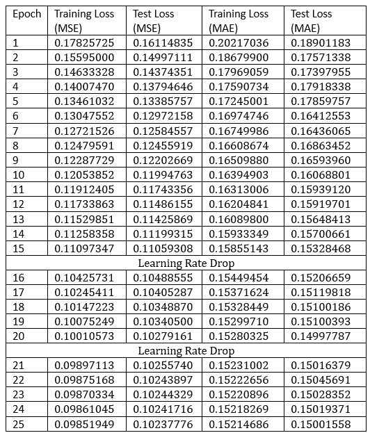
The learning rate was dropped twice to speed up convergence at higher epochs with the intention that the model would find the local minimum after these learning rate drops in their respective areas. The final result after 25 epochs was around 0.15 for MAE test loss.
4.4 Comparison to Baseline
While the baseline model and the final model used increasingly similar methods, the final model outperformed the baseline regarding the overall competition metric of MAE test loss (roughly a 8.5% reduction in test loss). With a higher number of epochs at the Optuna-defined learning rate, it is possible that the final model could improve the MAE test loss further, but the model was not tested any further than that due to computational time limitations.
4.5 Final Model Limitations
One aspect notable from the baseline model is its shorter runtime, as the baseline model efficiently runs each epoch in roughly 5.5 minutes. The current final model implementation takes around 9-10 minutes (close to double the time) per epoch. Additionally, the baseline model outperforms the current final model after being modified to optimize the mean squared error likely due to the baseline model utilizing a different learning rate scheduler where the learning rates gradually change rather than step-wise which would result in significantly more progress in reducing test loss. The final model also required prefiltering based on signal-to-noise whereas the baseline actively filters from the input file.
5. Conclusion
This project has successfully demonstrated the effectiveness of an encoder-only transformer model in predicting RNA nucleotide reactivity. By utilizing the self-attention mechanism and positional encodings, the model adeptly captures long-range dependencies within RNA sequences, showcasing a marked improvement over conventional methods. This achievement underscores the potential and applicability of deep learning techniques in RNA-related research, offering a novel approach to understanding the complexities of RNA structures and their reactive behaviors.
6. Future Work
6.1 Hybrid Models Development
The potential of combining the transformer model with other models, like graph neural networks, presents an exciting avenue for research. Such hybrid models could offer a more nuanced understanding of RNA structures, especially in representing complex tertiary formations that are pivotal in many biological processes.
6.2 Model Optimization and Scaling
As the complexity and size of datasets increase, optimizing the computational efficiency of the model becomes crucial. Investigating more efficient computational frameworks and algorithms will be key to handling larger datasets and more intricate RNA structures. Moreover, leveraging distributed and parallel computing frameworks could scale the model's application to larger-scale, real-world scenarios. A scheduled learning rate is one optimization tool that should be implemented in future iterations to ensure that the model efficiently converges.
Through these future directions, the project aims not only to advance the scientific understanding of RNA but also to contribute meaningfully to the broader field of molecular biology, paving the way for innovative solutions in healthcare and therapeutics.
References
[1] R. Das, S. He, R. Huang, J. Townley, R. Kretsch, T. Karagianes, J. Nicol, G. Nye, C. Choe, J. Romano, M. Demkin, W. Reade and Eterna players , "Stanford Ribonanza RNA Folding," Kaggle, 2023. [Online]. Available: https://www.kaggle.com/competitions/stanford-ribonanza-rna-folding/overview. [Accessed 27 November 2023].
[2] David Mitchell, Jennifer Cotter, Irfana Saleem, Anthony M Mustoe, Mutation signature filtering enables high-fidelity RNA structure probing at all four nucleobases with DMS, Nucleic Acids Research, Volume 51, Issue 16, 8 September 2023, Pages 8744–8757, https://doi.org/10.1093/nar/gkad522
[3] M. Szikszai, M. J. Wise, A. Datta, M. Ward, and D. H. Mathews, “Deep learning models for RNA secondary structure prediction (probably) do not generalize across families,” Bioinformatics, vol. 38, no. 16, pp. 3892–3899, Jun. 2022, doi: https://doi.org/10.1093/bioinformatics/btac415.
[4] Tycho Marinus, Adam B Fessler, Craig A Ogle, Danny Incarnato, A novel SHAPE reagent enables the analysis of RNA structure in living cells with unprecedented accuracy, Nucleic Acids Research, Volume 49, Issue 6, 6 April 2021, Page e34, https://doi.org/10.1093/nar/gkaa1255
[5] Busan S, Weeks KM. Accurate detection of chemical modifications in RNA by mutational profiling (MaP) with ShapeMapper 2. RNA. 2018 Feb;24(2):143-148. doi: 10.1261/rna.061945.117. Epub 2017 Nov 7. PMID: 29114018; PMCID: PMC5769742.
[6] Kengo Sato, Michiaki Hamada, Recent trends in RNA informatics: a review of machine learning and deep learning for RNA secondary structure prediction and RNA drug discovery, Briefings in Bioinformatics, Volume 24, Issue 4, July 2023, bbad186, https://doi.org/10.1093/bib/bbad186
[7] J. Zhang, Y. Fei, L. Sun, and Qiangfeng Cliff Zhang, “Advances and opportunities in RNA structure experimental determination and computational modeling,” Nature Methods, vol. 19, no. 10, pp. 1193–1207, Oct. 2022, doi: https://doi.org/10.1038/s41592-022-01623-y.
[8] W. Wang et al., “trRosettaRNA: automated prediction of RNA 3D structure with transformer network,” Nature Communications, vol. 14, no. 1, Nov. 2023, doi: https://doi.org/10.1038/s41467-023-42528-4.
[9] Franke, F. Runge, and F. Hutter, “Scalable Deep Learning for RNA Secondary Structure Prediction,” arXiv.org, July 2023. doi: https://doi.org/10.48550/arXiv.2307.10073.
[10] S. He, B. Gao, R. Sabnis, and Q. Sun, “RNAdegformer: accurate prediction of mRNA degradation at nucleotide resolution with deep learning,” Briefings in Bioinformatics, vol. 24, no. 1, Jan. 2023, doi: https://doi.org/10.1093/bib/bbac581.
[11] Mehdi Saman Booy, A. Ilin, and Pekka Orponen, “RNA secondary structure prediction with convolutional neural networks,” BMC Bioinformatics, vol. 23, no. 1, Feb. 2022, doi: https://doi.org/10.1186/s12859-021-04540-7.
[12] Muhammad Nabeel Asim et al., “EL-RMLocNet: An explainable LSTM network for RNA-associated multi-compartment localization prediction,” Computational and Structural Biotechnology Journal, vol. 20, pp. 3986–4002, Jan. 2022, doi: https://doi.org/10.1016/j.csbj.2022.07.031.
[13] Sanghyuk Roy Choi and M. Lee, “Transformer Architecture and Attention Mechanisms in Genome Data Analysis: A Comprehensive Review,” Biology, vol. 12, no. 7, pp. 1033–1033, Jul. 2023, doi: https://doi.org/10.3390/biology12071033
[14] A. Jaokar, “Understanding transformers from first principles - #artificialintelligence #115,” LinkedIn, https://www.linkedin.com/pulse/understanding-transformers-from-first-principles-115-ajit-jaokar/ [Accessed Dec. 4, 2023]
[15] Data augmentation, “Data augmentation,” TensorFlow, 2023. https://www.tensorflow.org/tutorials/images/data_augmentation#:~:text=Data augmentation will happen asynchronously,with data preprocessing%2C using Dataset. [Accessed Dec. 05, 2023].
[16] R. Agarwal, “Complete Guide to the Adam Optimization Algorithm | Built In,” Complete Guide to the Adam Optimization Algorithm. Accessed: Dec. 05, 2023. [Online]. Available: https://builtin.com/machine-learning/adam-optimization
[17] Iafoss, “RNA starter [0.186 LB],” RNA starter [0.186 LB]. Accessed: Dec. 04, 2023. [Online]. Available: https://kaggle.com/code/iafoss/rna-starter-0-186-lb
Appendix
Table 4: Baseline model modified to output MSE loss [17]
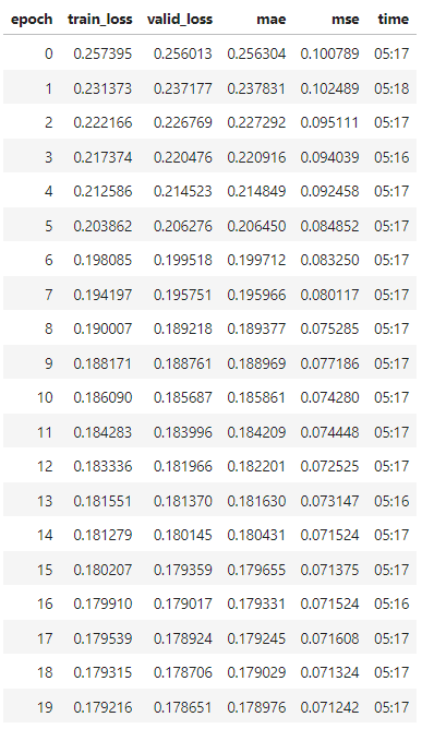
Table 5: Baseline model without modifications after 25 epochs [17].
